### Life 708
***
# Identifying Variation
***
### Will Rowe
View the presentation online at:
[will-rowe.github.io/identifying-variation-2017](https://will-rowe.github.io/identifying-variation-2017)
---
## Aims of these slides
***
* introduction to genome variation
* short read alignment
* interpreting alignments
* calling variants
----
## Introduction
***
**genome variation** = differences in DNA content / structure between two organisms
---
### Why look at variation?
***
* allows us to study evolution
- phylogenetics
- population genomics
* let's us make genotype / phenotype associations
- genome wide association studies (GWAS)
- human disease, agriculture, genetic engineering
---
### What is variation?
***
* Single Nucleotide Polymorphisms (SNPs)
- a genetic "typo" of one nucleotide (e.g. A > G)
* INsertion / DELetions (INDELs)
- a string of one or more nucleotides that has been added/removed from a location in a genome (typically 1-100bp)
* Structural Variants (SVs)
- a region of DNA that has been inverted / translocated / duplicated (typically >100bp)
* Mobile Genetic Elements (MGEs)
- insertion / replication of retrotransposons, transposons, integrons etc.
---
### How do we identify variation?
***
* Assembly and comparative genomics (eg. BLAST / ACT) good for identifying SVs and MGEs
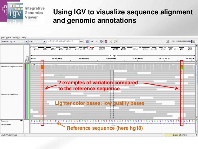
* Comparison of sample DNA to a reference allows identification of variation at a given genomic position
* Sequencing reads from a sample are **aligned** against a reference genome
* A **pileup** of the reads is essentially a sample of all the alleles present in the sampled cell population
- greater sequencing coverage = bigger sample size = greater certainty in variant calls
- considerations must be made for ploidy, sequencing quality / errors etc.
---
----
## Short Read Alignment
***
* To call variants in a sample, we need to align sequencing reads to a reference genome
* As discussed in previous lectures, we may have millions of short reads and a large reference genome (millions / billions of nucleotides)
* How do you align reads on this scale, in a reasonable amount of time / memory whilst allowing for inexact matching / errors?
* Other considerations also include: appropriate reference genomes, orientation / pairing of reads, multiple matching
* Short read alignment is hard as the shorter the read, the less likely a unique match to the reference
---
Computationally, exact matching is relatively easy:
```
READ 1: ATTCTTTACGACGAGTG
REFERENCE: AGCGTGACATTCTTTACGACGAGTGATATTCTGTAATAT
MATCH: *****************
```
***
Inexact (fuzzy) matching is much harder:
```
READ 2: ATTCTGTAAGAC
REFERENCE: AGCGTGACATTCTTTACGACGAGTGATATTCTGTAATAT
MATCH: *****G**A*** *********G*C
```
---
### Short Read Alignment
***
* There is an important distinction between read **mapping** and read **alignment**
- mapping is to quickly determine the best locations in the genome that a read could align
- alignment is to determine the best per-base alignment of a read to each possible mapping location in the genome
* Short read alignment is **global** with respect to the read and **local** with respect to the reference
- ideally the whole read matches one location in the reference genome
- in reality, repeats, variation and sequencing error add complexity
---
### Approaches to short read alignment
***
* A brute force approach would involve looking at every position in a reference for a possible query match
- this is not efficient
- indexing the reference so we know where possible matches occur improves the efficiency
* Hash-based indexing
- hashing of either the sequencing reads or the reference genome
* Indexing of trie structures
- utilising a reference index that is derived from a trie data structure
---
### Hash-based alignment
***
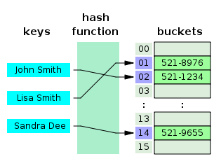
* Reads or reference sequence split into k-mers
* A hash function is used to convert k-mer strings to integers
* The integers are used as an array index for fast searching of the query sequence(s)
---
### Hash-based alignment
***
* Once the index has been built, the query is split into k-mers
- lookup query k-mer locations in the reference via the index
- for each query, select the reference location with most k-mer hits and perform Smith-Waterman alignment of read/reference (dynamic programming)
- this is the **seed** and **extend** principle
* The MAQ and SHRiMP short read aligners are based on this approach
- hash index the reads, scan using the reference sequence and use mapping quality scores to determine best alignments
- allowing seed mismatches and a spaced-seed approach is used to improve seed-matching sensitivity
---

---
### Hash-based alignment
***
* Hash-based approaches have some downsides
- static table means resizing can be costly - bad for a dynamic reference
- search performance reduces when reaching table capacity
* Majority of modern short-read aligners are **suffix/prefix trie**-based aligners
- main advantage over hash-based is that alignment of identical sequences is only done once
- memory footprint can also be much lower than hash-based approach
---
### Indexing of trie structures
***
* A trie is a computational data structure
- advantages of this structure include: fast lookup, no need for hash functions, no key collisions
* For short read alignment, the trie structure holds all the suffixes of a reference sequence as an index
- one trie node per common suffix
- this enables fast string matching (query look up)
---

* Example suffix trie for the text BANANAS
- all suffixes of BANANAS are found in the trie
- search for substrings by starting at the root and following matches down the tree until exhausted
- the paths of this trie can be compressed by removing nodes with single descendants
---
### Algorithms based on suffix/prefix tries
***
* these algorithms find exact matches and build inexact alignments (supported by the matches)
* to identify exact matches, the algorithms use a representation of the suffix/prefix trie
- E.G. suffix tree, suffix array, FM-index
- a special terminal character ($) is used to denote the end of the suffix
- FM-index is widely used due to it's small memory footprint
---

Suffix Trie ----- Suffix Tree ----- Suffix Array ----- FM Index
---
### The FM-index
***
* The FM-index is used by short read aligners such as Bowtie and BWA
* To understand how the FM-index is queried during read alignment, let's first look at the **Burrows-Wheeler Transform**
* The Burrows-Wheeler Transform (BWT) was originally a method to improve algorithmic efficiency of text compression but is widely used in bioinformatics software
---
### The Burrows-Wheeler Transform
***
* for a given reference sequence, T
* get all rotations of T
* form the Burrows-Wheeler Matrix (BWM)
* sort the BWM lexicographically
* the last column of the sorted matrix is the BWT of the reference, i.e. BWT(T)
---
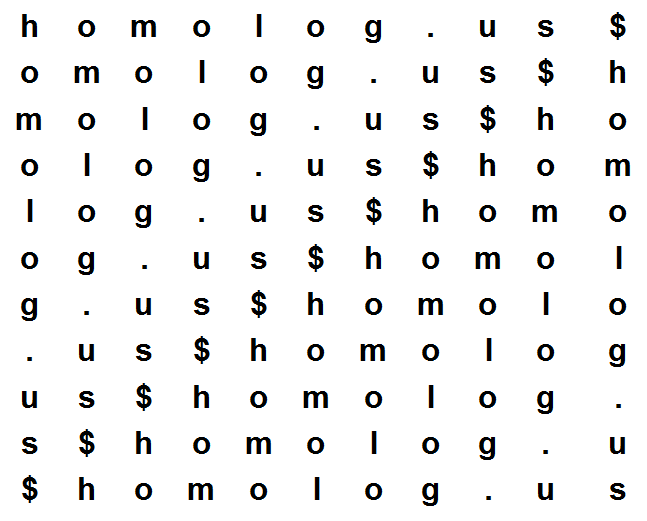
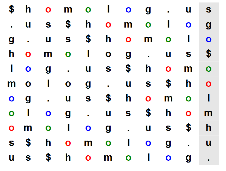
* get all rotations of the string "homolog.us"
---
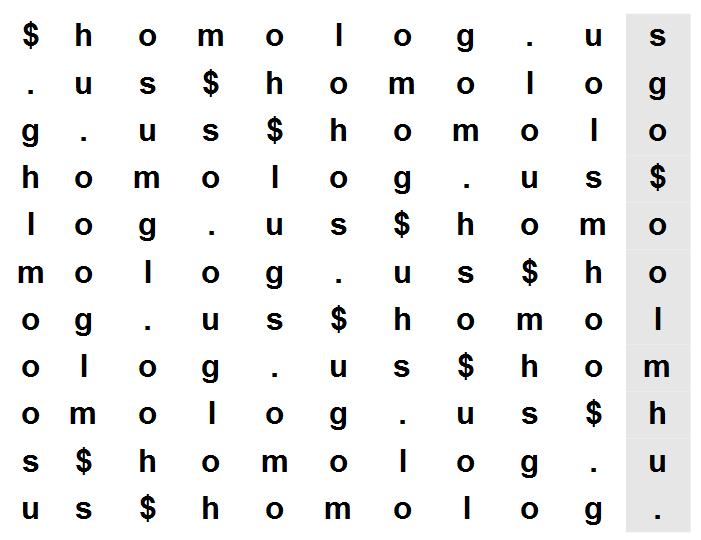
* sort the BWM lexicographically and look at the last column
---
### The Burrows-Wheeler Transform (BWT)
***
* The BWT of a string allows for efficient compression
- runs of the same character can be condensed
- this is what computing tools such as bzip2 are based on
- the BWM is not stored - only the BWT is used
* The BWM resembles the suffix array
- sorted order is the same, regardless if using rotations or suffixes
- this means, rather than finding all rotations, we can generate BWT(T) by:
```python
if SA[i] > 0:
BWT[i] = T[SA[i] - 1]
if SA[i] == 0:
BWT[i] = $
```
---

BWT = the characters one to the left of the suffixes in suffix array
---
### The Burrows-Wheeler Transform (BWT)
***
* The BWT is reversible - you can get the original reference sequence back
* For this we utilise the **Last-to-Front** (LF) mapping property
* This property means that the order of characters in the first column is the same as that of the last column
* Let's look at the homolog.us BWM example with all O's coloured by occurrence
---
---

---
### The Burrows-Wheeler Transform (BWT)
***
* Now that we have seen:
- how to perform the BWT
- how BWT can be used to compress a string
- how BWT can be reversed
* How is it used as an index in short read alignment?
- the **FM Index** allows for this and is based on BWT
---
### The FM Index
***
* Stands for Full-text Minute-space
* FM index combines BWT with a few additional data structures
- checkpoints and a suffix array sample
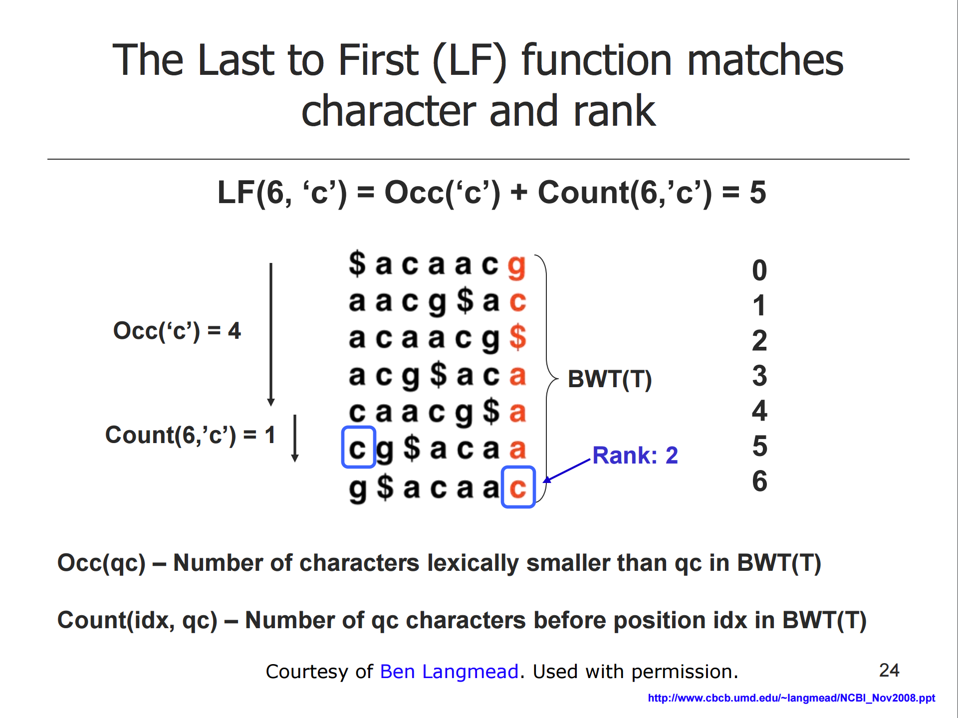
* Querying the FM index is based on the LF property
- the LF function matches character and rank
- this can be used to reconstruct T from BWT(T) or to query the reference
- the FM index stores extra information to facilitate this calculation
---
---
### The Burrows-Wheeler Transform (BWT)
***
* We have seen how the FM index can be used to find exact sequence matches
- requires small amount of memory
- short read alignment needs allowances for mismatches and read quality etc.
- solutions such as backtracking quality-aware searching facilitate this
* For more information on BWT, [this](http://www.cs.jhu.edu/~langmea/resources/lecture_notes/bwt_and_fm_index.pdf) lecture series by Ben Langmead is highly recommended
* For how it is implemented in short read aligners, [this](https://www.ncbi.nlm.nih.gov/pmc/articles/PMC2943993/#!po=25.0000) review and [this](https://arxiv.org/abs/1303.3997) paper are good resources
----
## Alignments
***
* Now that we know the basic principles behind short read aligners, let's go over the alignment results
* There is a single unified file format for storing read alignments to a reference genome called **SAM** format
* SAM stands for Sequence Alignment Map
- there is a binary version of this file format: **BAM**
- BAM allows for fast processing/indexing of the alignment
- there is also **CRAM** format (not discussed further) that offers reference-based compression
* We will explore the SAM format during the practical and use **samtools** to get basic alignment statistcs, as well as manipulate and convert alignment files
---
### Alignment Post-processing
***
* Sorting, filtering and indexing the alignment
- speeds up downstream analysis and reduces file size
- can be done using piped commands (holding alignment in memory)
* Local realignment
- InDels can cause reads not to align correctly
- multiple sequence alignment is performed in suspect alignment regions
* Duplicate removal
- duplicate reads may be PCR artifacts and these need to be marked/removed so that variant call is not biased (reduces false positives)
* Base quality score recalibration
- per-base recalibration uses reported quality score, read position and dinucleotide context
---
### Variant Calling
***
* To call variants from a pileup of reads, we generally use a probabilistic method (e.g. Bayesian model)
- tools such as Freebayes, GATK HaplotypeCaller, Samtools/BCFtools and Varscan are commonly used
* These programs calculate **genotype likelihoods** at each base position
- variants can be called relative to multiple samples
* Mapping quality, base quality and read pair information etc. is utilised in making the calls
* Variant calls are contained in a Variant Call Format (VCF) file
---
### Variant Filtering
***
* Once we have a VCF file, we apply filtering to reduce false positives
* We can filter using criteria such as depth, variant frequency, strand balance
* We could also use information on known variants to recalibrate our variant quality scores
* Once filtered, we should interpret our results and then see if we need to reapply the filters
- check SNP density, transition/transversion ratio etc.
---

----
## References
***
* [IGV](http://everythingcomputerscience.com/images/phone_book_HashTable.jpg)
* [suffix tries](http://marknelson.us/1996/08/01/suffix-trees/)
* [langmead lab](http://www.cs.jhu.edu/~langmea/resources/lecture_notes/bwt_and_fm_index.pdf)
* [homolog.us](http://homolog.us/Tutorials)
* GATK
* A survey of sequence alignment algorithms for next-generation sequencing. Brief Bioinform. 2010 Sep;11(5):473-83. doi: 10.1093/bib/bbq015. Epub 2010 May 11.
* Ultrafast and memory-efficient alignment of short DNA sequences to the human genome. Genome Biol 10: R25 Article in Genome biology 10(3):R25 · April 2009